Activity 9 - Volumetrics

Introduction:
Using UAS technology to collect and process volumetric data is one of the biggest advancements and arguments for using UAS. The ability to fly over an area, take a series of images and then process that area is not only efficient but accurate when using the correct methods. There are a number of figures that can be calculated including volume, surface area, elevation levels, etc. For the purpose of this lab volume is what is being focused on. There are a number of reasons a company may want volumetric data. Knowing the volume of a given area can be very important for the purpose of logistics. When dealing with mines it is important to know how much material is in a given area for calculating costs for processing the material and figuring out the amount of trucks or train cars required to move that amount of material. It is also crucial in scenarios where contractors are paid on a material moved basis. Often times these kinds of calculations are made every month to monitor efficiency and the overall level of product moved. Due to the fact these measurements are often done on a frequent basis there is a recurring cost each time, with most methods this cost is significant. There are a number of methods used to calculate the data including the use of a surveying team, LIDAR and also UAS. Doing volumetric calculations with a UAS is not only cost effective but also worker safety is improved because in areas such as open pit mines there is no longer a need for a surveying crew to walk around risking injury. Calculating volumetric data using a UAS can be done through several methods and programs. Perhaps the quickest and most straightforward method being Pix4D but ArcMap along with a set of tools can be used to also calculate volumes.

Methods:

Volume from Raster
Using ArcMap there are a couple of methods used to calculate volumetric data. The first being the use of 3D analyst to calculate the volume of a raster clip. To do so requires a number of tools and steps. The first step being creating a polygon feature class. When doing volumetric calculations it is important to focus on just the area you want to gather the data on. For this instance, volumetric data was calculated on three separate "piles" of material. When creating a feature class for each pile it is important to include just the intended pile, if the polygon includes other piles or the intended pile is cut off, the data cannot be considered accurate. Once the piles are defined (Figure 1) it is time to "Extract by Mask" this is essentially used to eliminate all the rest of the area surrounding the piles as it is not required for calculating the data. Once each feature is extracted only the intended areas will be left (Figure 2).

Figure 1 - Masked polygons at Litchfield Mine site.

Figure 2 - Extracted Piles

Once you have the piles separated the next step is taking note of the elevation by using the "Identify" tool (Figure 3). This step is crucial as the elevation for each pile area is needed for the next tool.

Figure 3 - Identify Tool Symbol

The final step for calculating volume using a raster using the "Surface Volume" tool (Figure 4). This tool is essentially calculating the area and volume between a surface and reference plane. In the case of this lab, the reference plane is the polygon surrounding the pile. For this tool to work the elevation or Z value needs to be inserted. Once the tool is finished, a text file with the volume of the pile is saved to the designated folder path.

Figure 4 - Surface Volume tool 

The model below (Figure 5) shows the entire process needed to calculate volume using a raster.

Figure 5 - Volume from a raster model

Volume from TIN
The next method of calculating volume is using ArcMap and using a TIN. TIN stands for Triangulated Irregular Network.  The first step is taking the raster clips created in the previous method and converting those using the "Raster to TIN" tool (Figure 6). A TIN contains better surface definition because of the use of triangulations. (Figure 7) Once the tool finishes, the next step is using the "Add Surface Information" tool (Figure 8) on each TIN, specifically adding the "Z_Mean" value. This tool is useful because in general, elevation values are usually ignored in ArcMap unless requested by using tools such as this.

Figure 6 - Raster to TIN tool

Figure 7 - Image featuring converted TINs

Figure 8 - Add Surface Information tool

The last step in calculating the volume is using the "Polygon Volume" tool. The reason "Surface Volume" tool isn't used is because it isn't designed for TIN features and "Polygon Volume" (Figure 9) takes the average surface elevation added using the "Add Surface Information" tool. The volume can now be found once clicking the pile using the "Identify" tool.

Figure 9 - Polygon Volume tool

The model below (Figure 10) shows the entire process needed to calculate volume using a TIN.

Figure 10 - Complete TIN volume model

Volume from Pix4D
The final method explored in this lab is the use of a program that had been used in previous labs but specifically back in Activity 7 where the volume of a pavilion was found.
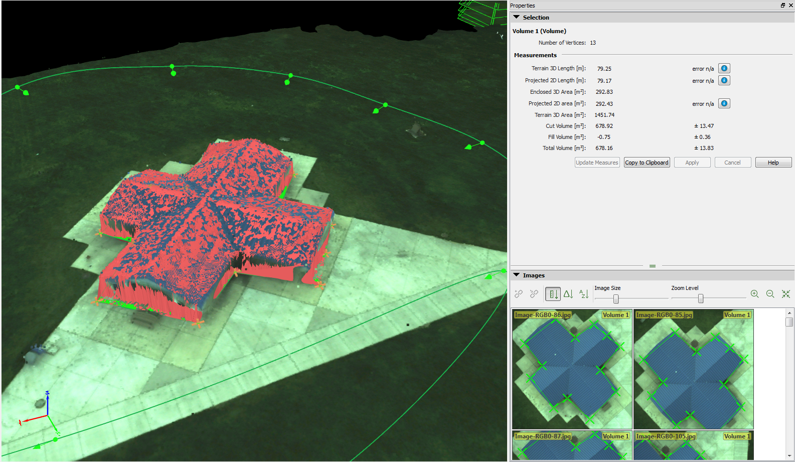
The process for calculating volume in Pix4D is extremely simple. At the top menu bar there is a "Measure" area, from there select volume. Using the tool, select points around the base of the area or in this case, pile, until the area is completely enclosed like in (Figure 11). Once complete, click "Calculate Values" and the volume of your selected area will be presented.

Figure 11 - Calculating Volume in Pix4D

Results

Looking at the table (Figure 10) there are some differences in results. The raster volume compared to the Pix4D volume results are closest. It makes sense the raster volumes are the highest because while doing this method, volume from the surrounding area may end up included in the result. In essence, volume is overestimated slightly.

The TIN volumes are way off and it makes sense given the default values used. When calculating the TIN, the default value of 1,500,000 maximum points was selected. This makes the process relatively quick but as the table shows, much less accurate. If a value of 15,000,000 or even 25,000,000 points was selected the data would be much more accurate but take longer to calculate. With 1,5000,000 the polygon was very simple and not detailed like the actual pile would be.

As far as accuracy goes, doing the raster method or Pix4D method will produce the best results. If time is an issue, Pix4D is a clear winner. Although there aren't as many steps to the Raster method compared to the TIN method the Raster method took longer to process but produced more accurate results. Doing the Pix4D methods seems like the best overall way. The sheer level of simplicity really highlights how powerful the program is and is just one of many tasks it can handle in an efficient matter.

Conclusion
When using UAS to calculate volumes there are many methods possible. Picking the right one really depends on the project at hand and what resources are at your disposal. As with most data processing, the higher specifications your computer has the faster and more efficient the data will be processed. Not every company has Pix4D available, in that case, programs such as ArcMap can be used to supplement and still get accurate results. In a professional setting where money is being exchanged and accuracy is key it is important to be diligent and triple check results to make sure both parties are happy with the results. In the case of open pit mines, using UAS is a perfect method. UAS in a mining situation is efficient, cost effective, improves safety, and accurate.

Activity 8 - Adding GCPs to Pix4D Software

Introduction/Overview:
     In the previous lab, a brief introduction to the software package known as Pix4D was given. In this lab further exploration of Pix4D is done. The focus of this lab is to utilize GCPs or Ground Control Points in order to get the most precise data for our model and mosaic. The GCPs increase accuracy and overall quality.

     Pix4D is an extremely user friendly program and the leader in software for constructing point clouds. In this lab the data being processed was imagery taken back during Field Activity #4. Over 300 images were taken with the Canon SX260 and the equipment we used to gather GPS data at our GCPs was a Topcon Positioning System.

Methodology:

     To collect the data we used a combination of the Matrix UAS and Canon SX260 at a height of 70m. To fly the area we used Mission Planner and as mentioned earlier to gather the GPS dating of our GCPs a Topcon Positioning System was used. The data was then processed with Pix4D and also supported with ESRI programs such as ArcMap.

     When using Pix4D there are numerous ways to incorporate and use GCPs when processing imagery. GCPs can be measured while being out in the field such as using surveying equipment, brought in from existing data and also gathered from a Web Map Service such as Google Earth.

       If your sensor does not geolocate images it does not necessarily mean you can't run the data. Through the use of GCPs we can tie this data in to our imagery and get an accurate image. Pix4D allows for a couple of methods for adding GCPs to images. The first method (Figure 1) is designed when the GCPs have a coordinate system known.

Figure 1 - Method 1 for adding GCP data to your images

The next method (Figure 2) can be used in a couple of instances including, your initial images are lacking geolocation, the initial images are geolocated in a local system and lastly, the GCPs are in a local coordinate system.

Figure 2 - Method 2 for adding GCP data to your images

The last method is really a coverall way (Figure 3). Regardless of the various coordinate images your data has Pix4D will process the data it will just take longer but can be started and does not have to be babysat during the process unlike the other two. **Try to avoid unless time is no constraint.

Figure 3 - Method 3 for adding GCP data to your images

     In addition to knowing what method to incorporate GCPs through it is also essential you select the correct coordinate system. The coordinate system for our GCPs were NAD1983 Zone 15 so that is what needed to be selected. In addition, it is important to note your output coordinate system should also be the same as the GCPs. The default for image coordinate systems is WGS1984 but with Pix4D the image and GCP coordinate systems do not have to be the same.

     Following the same basic sequence as the previous lab, images were loaded in to Pix4D. Although the images were geolocated we had GCP data and the coordinate system was known. Going off of that, Method 1 (Figure1) was used in order to add GCPs to the project. The program prompted a coordinate system to be selected and this is where NAD 1983 Zone 15 was chosen. The GCP/Manual Tie Point Manager (Figure 4) is a tool that shows the user the coordinates of each GCP and how many tie points have been manually adjusted. Once the GCPs are added run Step 1: Initial Processing, after that is a complete look at the Initial Processing Report and begin marking tie points. To tie points to the GCP a user has to go under rayCloud Editor and manually select tie points near the center of the GCP (Figure 5). Accuracy is based on the number of "ties" a GCP gets and for this lab at least 10 images were "tied".

Figure 4 - GCP/Manual Tie Point Manager showing how many tie points and location of each of our 6 GCPs

Figure 5 - Example of adding "ties" to images of GCP 5.

      Once the GCPs are tagged the image is prepped to be ran through steps 3 and 4. These steps can take anywhere from a couple of hours to a couple of days depending on how many images and GCPs the project has. It is crucial you make sure everything is set and ready to go before running the rest because you could potentially throwing out a lot of processing hours if do not select the right things. A good way to check your progress before running the last 2 steps is to examine the Initial Processing Report (Linked below). It addresses items such as quality check which essentially gives you an idea of how many images the project contains along with a some georeferencing and matching stats. There is also a preview included which is a glimpse of what is to come. If the preview is off, make sure you take care of what is missing before continuing. Also included are image position locations, GPS tie points, the amount of overlap and an overview of geolocation details which shows the level of error.

     For the sake of comparison the data was also processed without the addition of GCPs added. The results of the initial processing report for that can also be found linked below.

Initial Processing W/GCP
Initial Processing W/Out GCP

Results:
     Once the processing is complete you will be presented with a Final Report (Linked Below). This report expands upon the original Initial Report and updates needed values. As you can see the project containing GCPs has a much increased accuracy with drastically less amounts of error. The project with no GCPs has the same accuracy as the initial process states because the geolocation was not improved upon.

Final Report W/GCP
Final Report W/Out GCP

     Pix4D Also creates .tiff images that can be brought in to ArcMap. These can be placed over basemaps to give an updated image of your study area. This is where location accuracy is crucial. (Figure 6) shows the .tiff containing GCP data while (Figure 7) highlights what happens when your data integrity is not at it's fullest. As you can see in (Figure 7) the imagery tends to pull towards the Northeast, something adding GCPs corrected.

Figure 6 - Map with GCP data

Figure 7 - Map without GCP data

     A simple .gif image (Figure 8) comparing the two .tiff images is a decent indicator of the differences between the two. Although some may consider the differences minimal, when you are working with images that need to be geolocated correctly, a few meters is like night and day.

Similar to Pix4D in ArcScene, you can also "explore" the 3D model once adjusting the base heights for both the .tiff (Figure 9)  and .dsm. (Figure 10). These models give you an idea of the varying levels of elevation.

Figure 9 - .tiff with adjusted base heights in ArcScene 

Figure 10 - .dsm with adjusted bas heights in ArcScene

     Much like the last lab you can also "tour" your finished product. Below (Figure 11) is a tour highlighting each of the 6 GCP locations and also the study area as a whole.

Figure 11 - Video tour of 3D model created in Pix4D

While collecting data that day we also used a variety of other methods to see how accurate they were compared to the GCPs we laid out (Figure 12).

     There is truly so many ways the data can be manipulated and further processed but the above were a few key, basic items. All came from ArcMap, ArcScene, Pix4D.
Conclusion:


Again, Pix4D claims to be user friendly and the "help" guide proves itself time after time. If don't with time and care GCPs can be added in an efficient matter and can drastically improve the quality of your image. When adding "ties" the more you add the more "self aware" Pix4D gets and it begins adding ties for you. Alone, the SX260 does a decent job with geolocating but it is not at survey grade. This is why proper equipment and diligence is so important when working with precise imagery. This is still only scratching the surface of what Pix4D has to offer but going forward with the knowledge in regards to GCPs, our images will only improve with accuracy and the quality of the finished product will also improve.

Activity 7 - Pix4D

Overview:

     In past labs georeferenced mosaics have been mentioned but until now they have never been a true orthomosaic. Fortunately, Pix4D a UAS mapping software packages makes creating these extremely easy, and accurately. Although easy to navigate this software demands a lot of computer resources to process data quickly and has some guidelines such as in general your images should have 85% frontal overlap and at the very least 70% side overlap to be safe. Some terrains are more difficult than others such as snow and sand, to achieve the best results at least 85% frontal and 70% side overlap but also try and get adjust the exposure settings. With the right exposure you will be able to get the most contrast from each image.  Depending on the specs of your computer and how many images you are processing determines the time it will take to finish. Luckily, Pix4D includes a feature that allows you to view a preview, they refer to this feature as Rapid Check. This can save countless hours incase your data is not good and you wait for it to process sometimes for 12+ hours at a time. Rapid Check works by reducing the resolution of all your images to 1 mega pixel. This gives you not only a preview but gives you an idea of the quality level of your images. Whether or not the Rapid Check succeeds or fails is an indicator if you should move on with the project or collect data again achieving more overlap or a different method. Pix4D is also capable of handling multiple flights at a time. To do so the pilot has to make sure there is enough overlap and conditions remain as close as possible. For example, weather, sun direction, altitude, etc all need to be considered when handling multiple flights. While using Pix4D you are not just limited to using images shot in nadir, oblique images can also be used but there should be images taken from the ground as well and if you are capturing flat ground, nadir is recommended. Depending on your project you may want to use GCPs although these are generally optional. GCPs can be used to improve accuracy and is important to use if your sensor does not geolocate. During the various steps of processing a quality report is written. This gives the user an idea regarding the level of quality their project and if there are errors, what needs to be done in order to fix those errors.

Walkthrough:

     Although very user friendly Pix4D is a very powerful program with many uses. For this lab a very basic project was processed in order to introduce us to Pix4D and get us accustomed to the basic features. For this lab all of the images used were shot in nadir and it is important to note we did not use GCPs.

    When starting the program and a new project Pix4D prompts you to add images to begin processing. (Figure 1) Make sure to add all over your images in order to get a complete product.

Figure 1 - Adding Images to Pix4D

For this lab I processed two sets of images separately both featuring the Eau Claire Soccer Complex Pavilion shown in past labs.

     Once the images are added a screen will popup showing you the image properties. (Figure 2) Listed here are the coordinate system, if your images were geolocated or not and the camera/sensor used to take thos images. It is important to note, some sensors do not geolocate images and it is advised to supplement that through the use of GCPs or a georecording device that tracks points where images were taken.

Figure 2 - Image Properties Menu

     From there you are prompted with templates, this helps determine what direction you want to take the project. For this lab we went with the default 3D maps as you can see in (Figure 3)

Figure 3 - Project Template Selection

 

     Next, the processing begins, at this point its start and wait. Depending on the level of quality and number of images you have determines how long it will take for the entire process. The better of computer you have the less time it will take to process. Along the way, frequent process reports will pop up giving you quality updates and even previews of your final image/model.

     The quality report includes many useful things as mentioned earlier. One example is it shows you how many of your images were used in creating the finished product (Figure 4) and where your key areas of overlap were and were not. (Figure 5) In the case of the SX260 all of my images were used in creating the image.

Figure 4 - Beginning of Quality Report

Figure 5 - Overlap details

It makes sense my weakest areas of overlap were the outside fringes on the mission area. These areas were not the main focus of the mission therefor less images were meant to be taken.
     The first data I ran was from the Sony SX260, it was 32 images at 14 megapixels each. The SX260 geolocates images so I did not have to worry about that.  They were shot at 70m and in all it took around 30 minutes from start to finish to process. The other set of images I processed were taken by the GEMs sensor. There were 220 non-geolocated images so GPS data had to be added to maintain accuracy. Although there were many more images taken the GEMs only takes pictures at 1.3 mega pixels. This took slightly longer to process at around 40 minutes. The process for both the SX260 and the GEMs was nearly identical and consequently produced very similar results.

Post - Processed Data

     Once finished processing the data can be manipulated in a number of ways and almost "explored" much a like a virtual tour of the study area. A few of the basic features of Pix4D include, measuring features, find surface areas of objects and also some volumetrics. Because we are just getting introduced to Pix4D I used just those three tools. I measured the width of the sidewalk. (Figure 6), found the surface area of one of the soccer fields (Figure 7) and also the volume of the pavilion (Figure 8).

Figure 6 - Width of Sidewalk

Figure 7 - Surface Area of Soccer Field

Figure 8 - Volume of Pavilion

 You can also record an animation that "flys" you through the project. This is a relatively rough model given the fact we just used nadir images but gives a viewer a sense of the study area and can be made quickly. (Figure 9).

Figure 9 - Video Flyby Tour of GEMs 3D Model

With the processed data you are not restricted to just using the data in Pix4D. It can also be used and imported in to ArcMap. Here you can add metadata to your images, an important step in to ensuring data integrity. You can also create maps using the orthomosaic images  you created. (Figure 10, 11, 12)

Figure 10 - SX260 Orthomosaic made in ArcMap

Figure 11 - GEMs Orthomosaic made in ArcMap

Figure 12 - GEMs Orthomsaic with surface overlays from earlier calculations

Activity 6 - Post Processing

GEMs Sensor - Sentek System Product Review / Report

Basic Overview 
     For the longest time imaging using a UAV meant making sacrifices based on what sensor you had available. Often this meant mounting a camera in an unorthodox position and asking it to do things it wasn't made to do. This all changed with the GEMs sensor by Sentek System. This sensor is one of the first of it's kind, a sensor made specifically to be used with a UAV. GEMs stands for Geo-localization and Mosaicing System and it happens too do both quite effectively as you can see here. The GEMs manages to pack a dual 1.3 megapixel sensor into a very small form and includes GPS too geocode each image taken, an almost absolute must when it comes to effectively image an area. The Ground Sampling Distance or GSD is 5.1cm @ 400ft and 2.5cm at @ 200ft. These figures are important because with aerial imaging, location accuracy is key. Something that sets the GEMs apart from most sensors is the way images are stored. Most cameras use SD cards but the GEMs saves images to an external usb flash drive. Using a flash drive is nice because the cost associated with these is lower, they can write faster than most other storage formats and hold more data. Because the GEMs is lighter than most sensors (170 grams) and smaller it makes it possible to mount in even the smallest of spots but there are a couple of things to look out for and consider when placing the sensor especially on quadcopters. The biggest thing to remember is that the GEMs is meant to be placed downwards to the ground and flat to minimize distortion. Some other factors to consider is the amount of vibration the sensor experiences. If the sensor vibrates too much the accelerometers in the sensor can be thrown off, reducing the quality of your finished mosaic. Something else to watch out for is EMI or electromagnetic interference, luckily Sentek came out with a solution and includes shields on the sensor to prevent that from happening. When it comes to actually flying your mission and recording data there are some factors to consider. Each sensor is different and you have to find the perfect mix of height, speed of flight combined with your sensor specs to get the level of detail your project requires. When using mission planner software there are some things you need to input regarding sensor information. Fortunately, Sentek provides information pertinent to the GEMs for Mission Planning. (Figure A)

Figure A - Values to input in to Mission Planner for best results.

Software Overview

     There also happens to be a GEMs software package available for purchase or comes alongside with the GEMs sensor. The software takes your taken images from the usb drive along with GPS coordinates and according to Sentek Systems creates an orthomosaic of multiple forms including RGB, NDVI, NIR. In this case the GEMs software creates a georeferenced image which is great but is really only usable for measurements when GCPs (Field Activity 4) are used. Georeferenced Images

Using the Software

     Using the software is pretty easy. Locate the folder where your images are located and insert them in to the GEMs software. The software automatically names the folder in this format - " Fight Data (Week=X TOW=H-M-S). Where X, H, M, and S are numbers specifying the instant that data collection began for the associated flight. X is the GPS week number of the starting instant. H, M, and S represent the hours, minutes, and seconds, respectively, into the GPS week of the starting instant." Using converters this can be turned in to an exact time frame. Once locating the folder click "run" and click "NDVI Initialization" Once this is finished running it can be imported into various programs such as ArcMap which is what we used to look at and work with the data. Once processed, bringing .tif images in to Arc allows you to match up the data you collected with a basemap and essentially covers the old imagery allowing you to see an up to date image of the area you imaged. This format is needed because .jpeg images do not include geolocations, essential for GPS accuracy. One thing to note with the data brought in using the GEMs is that the data does not have metadata associated with is so the user, in this case (me) has to go in and edit the metadata to preserve data integrity and provide information so others can see things such as when the data was collected and how it was collected.

Types of Images

     The GEMs is unique in the sense that it doesn't limit you to just RGB and modded NIR. There are several formats included with the GEMs, RGB, NIR and NDVI.

RGB - Figure 1 - Represents true color, what the surface looks like with your naked eye.

Figure 1 - RGB Image

Monofine Image - Figure 2 - The fine NDVI mono shows the reflectance levels as a high to low. The GEMS software does not assign a color scheme to this NDVI. Healthy high reflectance areas are white and low health is gray to black.

Figure 2 - Mono Fine Image

NDVI FC 1 - Figure 3 -  Mainly used for monitoring vegetation, the red and orange representing vegetation and water content of that vegetation.

Figure 3 - NDVI - FC 1 Image

NDVI FC 2 - Figure 4 - Much like FC 1 except more visually appealing, where green represents vegetation much like the color of the vegetation. Red is min. NDVI while Green is max.

Figure 4 - NDVI - FC2 Image

Normal NDVI Mono - Figure 5 - Black represents min. NDVI while White is max. this colorway is mostly used for finding small plant growth found in soil throughout a large area.

Figure 5 - NDVI Mono Image

Flight Path - Figure 6 - This map shows the mission and path the Matrix Quadcopter took carrying the GEMs in order to image this particular area at the Eau Claire Soccer Complex.

Figure 6 - Flight Path

Final Critiques 

     Anytime you purchase a first generation device you have to be willing to accept there may be flaws and often a high upfront cost, especially when there are not many other options available specifically for this application. The GEMs sensor is no different. Alternatives to the GEMs Sensor are cheaper, but are not necesarily created for UAVs yet people have found ways to use them, avoiding the high price tag of the GEMs. To purchase the GEMs you have to contact Sentek Systems directly and they will assist you with purchasing. As stated on their website the GEMs is 100% designed, tested and manufactured in the United States.
     The price set aside the GEMs is a very capable sensor and does what Sentek claims it does. Although only 1.3 megapixel the images are clear and effective but for agricultural purposes this is good enough. I'm a little disappointed they did not include a better camera just knowing with how advanced phone cameras have gotten considering the size factor.  Sentek markets the sensor for agriculture and as you can see in the processed images here, it will do an effective job. As competitors enter the market and availability increases the cost of sensors such as the GEMs will decline.
     If you have the funds and do not want to fiddle with modifying other sensors to accomplish what the GEMs does it will serve you perfectly. The GEMs plugs directly in to the UAVs power and works fluidly. We did not have any issues with processing the data and it was very capable. I would recommend the GEMs Sensor as of right now and will revisit this review if I feel otherwise once processing data with the other sensors. It is a sensor made for UAVs and delivers what Sentek claims, the software it comes with pairs with the sensor and prepares the captured images in to .tifs in a timely matter.  

Activity 5 - Obliques for 3D - Model Construction

Introduction:
So far this semester we have been capturing our images in Nadir or straight down below the aerial device. This works well because the scale of the image remains relatively constant so measuring distances is possible. This week we focused on taking oblique images to process and create a 3D - model. Shooting oblique images means having a tilt of more than 3% and angled compared to nadir where the image is straight vertical down. The oblique images can be stitched together to form an accurate, explorable 3-D model. For this field outing we focused on collecting oblique images to create just that, a precise 3-D model.

Study Area:
This week our study area was the Eau Claire Sports Complex. We specifically focused on the imaging the pavilion found there (Figure 1). This was a familiar location to us but this time we focused on collecting a set of much different images for processing later this semester.

Figure 1 - Pavillion we focused on imaging

The weather during our outing was excellent with it being around 60 degrees, light cloud cover and low winds. There was mare tail clouds in the sky indicative of a storm coming but luckily we avoided any storms that were on their way.

Methods:
The first set of data we collected was done so by the use of the 3DR Iris + accompanied with a GoPro camera. The GoPro is great for capturing video but not ideal for this purpose because there are no geotags associated with each picture taken. This makes it more difficult to make a model out of the images because there is no GPS associated with the images. We will have to match up GPS points from the flight log with the images in order to create a decently accurate model. Using Mission Planner we created a mission plan that is referred to as a "structure scan" this meant the Iris + would autonomously fly itself around the building starting at 5m and gather images every 2 seconds capturing as many angles and views of the structure as possible. Upon doing so we decided that we need to gather images lower than 5m so we did so manually after the autonomous mission was complete. Although our model is not complete yet I will post it when done. Here is a .gif image (Figure 2) of our flight so you can see the number of passes and corkscrews the Iris + did to capture all the angles of the pavilion.

Figure 2 - All the images gathered using the Iris +

The next set of data we collected was using the DJI Phantom 3 Professional. The Phantom was a little more suited for doing this task because unlike the Iris, the Phantom does geotag each image you take making it much easier to create a model with after data processing. With the Phantom all of our images were gathered manually. We each got a chance to fly around the pavilion and gathered pictures every couple of seconds. The .gif image of our flight can be seen below (Figure 3)

Figure 3 - All the images gathered using the Phantom 3

It will be interesting to see the difference between the two models. The Iris was flown almost strictly autonomous with very precise movements and regularly spaced image capturing (every 2 seconds) while the Phantom was manually flown and the images were all taken by the pilot at an irregular time interval. While doing previous field activities we focused on capturing a broad area for the purpose of mapping while with this activity there was emphasis on one area and making sure we were extra thorough in gathering images of one structure.

Discussion / Results:
Before today the only images we had captured of the pavilion looked like this (Figure 4) as you can see our images only focused on the roof. Now using images such as this (Figure 5) we can put together a 3 - D model that focuses on all surfaces and sides of the pavilion. With capturing the roof it really only comes down to needing one image if capturing in nadir but with oblique it takes many passes and varying angled shots to capture the whole roof. Capturing oblique takes a lot more time to cover an entire surface but the level of detail is significantly higher. In previous field outings we've had a strong focus on mapping but with this exercise we weren't necessarily mapping but more so modeling.

Figure 4 - Vertical image taken from Field Activity #3

Figure 5 - One of many oblique images taken of all sides of the pavilion

Conclusion:
Using two different devices we captured the same structure. Using two different methods not only increases our chances at getting a successful model but also shows us there are varying ways to accomplish the same goal. Using GPS data or geotagged images we will be able to create a 3 - D model of a structure using image processing software. The applications for this are really endless, farmers could use the same methods to image their fields, insurance companies for disaster areas, the fire and police services could model crashes and fire scenes. Although capturing in oblique isn't as scale friendly and as easily measurable as nadir it serves a purpose especially when mapping. With nadir there is not as much distortion and oblique can show far more detail such as height. To do modeling using images oblique is necessary yet time consuming.

Activity 4 - Gathering Ground Control Points

Introduction:
The primary focus on this activity was to get the class accustomed to using Ground Control Points or GCPs as a way to georeference and be able to geometrically correct aerial images taken by a UAS. To get the utmost accuracy one has to be very careful with the methods and equipment used in collecting GCP data. To prove this point we used a plethora of devices with GPS recording capability and compared them. When using GCPs in an area a bare minimum of three points has to be used. The more points you use, the better your end data will be. If you area has a lot of topographic variance more points will be needed to accurately gather data for that area. When focusing on an area GCPs should be well spread out and one should avoid placing them on the edge of the desired area because the further you get away from the center the more an image is distorted.

Study Area:
For this activity we moved to a new area (Figure 1) not as cut and dry as the soccer fields we are used to.

Figure 1 - Highlighted area where we placed our GCPs, located south of South Middle School

Weather conditions that day were adequate for the task at the hand, it was sunny and remained in the low 60s.

There was some varying terrain but nothing more than some tall grass and some cut trails. We focused on covering the area around the small pond. If there was more variance in elevation we would have had to of used more GCPs. 

Methods: 
The first step was laying down our GCPs in different locations, for this area we placed 6 around the pond in different spots in the study area shown in (Figure 1). You can use a number of different items as markers but for this exercise we were lucky enough to survey marker mats (Figure 2). 

Figure 2 - Marker we used as a GCP

These markers were nice because they were all uniform is size and gave us an exact cross to focus on in the middle. Consistency is key with GCPs to keep a high level of data integrity.

For data collection we used a wide variety of methods each with varying levels of accuracy. 

The first tool we used was a Dual Frequency Survey Grade GPS, the level of accuracy with this is unmatched but it comes with a price, 12k for educational use and 18k for commercial. (Figure 3)

Figure 3 - Dual Frequency Survey Grade GPS 

With all the devices we used it was very important we took the reading from the same spot on the GCP as you can see above (Figure 3) Ethan took his time making sure the device was level and in the center of the GCP.

The next two devices we used were similar to one another just had varying levels of preciseness and also different costs respectively. Both were Bad Elf GPS just one was of survey grade (Figure 4) at $600 while the other (Figure 5) was at the enthusiast level at $125. We paired both of these with a tablet to record the data.

Figure 4 - Survey Grade Bad Elf

Figure 5 - Bad Elf GPS Pro

The next device we used was a basic Garmin GPS unit, these can be purchased for less than $100. They do not claim to be pinpoint accurate but are more so aimed at giving you a general idea of where you are. Nonetheless we used this device for the sake of comparison. 

Also for the sake of comparison, we used a smartphone in two different ways to show how truly inaccurate cell phone GPS is and how it should not be used in surveying or with CGPs. We used ArcCollector and the GPS data associated with images taken on an iPhone. 

Lastly, we drew up a mission on Mission Planner (Figure 6)  and used the Matrix Quad Copter to do aerial imaging. This data will be processed and I will post the results after that is completed.

Figure 6 - Mission Plan we used for aerial imaging with our GCPs below.

Discussion/Results:

The devices we used all had their pros and cons. Generally the more expensive and complicated the better results you will get. The Dual Frequency Survey Grade GPS was cumbersome and expensive but highly accurate. The Bad Elf GPS units were easy to use and cheaper but you sacrifice some accuracy with those trade offs. The last devices really have no place in the GCP world but were interesting to use and compare to the more specified devices. Our results of the comparison can be found below (Figure 7). 

Figure 7 - GPS Unit Comparison

You may think by glancing at this that they were all pretty close but when it comes to surveying and GCPs we want pinpoint accuracy and that is where the expensive, harder to use equipment really shines through. 

Surveying technology, like any other field is rapidly growing and more portable options with precise accuracy will only become more and more available. Although the Dual Frequency Survey Grade GPS is amazingly accurate it is bulky, takes an extra amount of time to use and could be difficult to use with different terrains. The Bad Elf on the other hand is small, portable, much cheaper and still fairly accurate. 

Gathering GCPs is time consuming because one must be very precise with GCP location selection and collecting the data. Depending on the area being analyzed many factors such as topography, weather conditions, foot traffic, etc all have to be considered. 

This activity relates to commercial practices in a few ways but mostly in the sense that these are the tools professionals are using today and to be successful in this industry you not only have to know how to accurately collect the data but processing it correctly is equally as important. 

GCPs are important whenever accuracy is paramount. As our readings say, the more GCPs you have the better the quality of data but you must have over 3. 

GCPs relate to UAS missions because they are used as a second form of measuring an area. When processing the aerial images, GCPs will come in very handy for verifying the calculations are correct and the data is valid. 

Conclusion:

Although sometimes time consuming and not nearly as thrilling as flying a UAS to collect data GCPs play a vital role in GPS data collection and verifying the information you collect is correct and as accurate as possible. Depending on the device you use the level of accuracy is directly related. When using GCPs you must have at least three markers and if your area has varying levels of elevation that all has to be considered. As technology improves collecting GCP data will get quicker and easier while remaining very accurate.