Activity 8 - Adding GCPs to Pix4D Software

Introduction/Overview:
     In the previous lab, a brief introduction to the software package known as Pix4D was given. In this lab further exploration of Pix4D is done. The focus of this lab is to utilize GCPs or Ground Control Points in order to get the most precise data for our model and mosaic. The GCPs increase accuracy and overall quality.

     Pix4D is an extremely user friendly program and the leader in software for constructing point clouds. In this lab the data being processed was imagery taken back during Field Activity #4. Over 300 images were taken with the Canon SX260 and the equipment we used to gather GPS data at our GCPs was a Topcon Positioning System.

Methodology:

     To collect the data we used a combination of the Matrix UAS and Canon SX260 at a height of 70m. To fly the area we used Mission Planner and as mentioned earlier to gather the GPS dating of our GCPs a Topcon Positioning System was used. The data was then processed with Pix4D and also supported with ESRI programs such as ArcMap.

     When using Pix4D there are numerous ways to incorporate and use GCPs when processing imagery. GCPs can be measured while being out in the field such as using surveying equipment, brought in from existing data and also gathered from a Web Map Service such as Google Earth.

       If your sensor does not geolocate images it does not necessarily mean you can't run the data. Through the use of GCPs we can tie this data in to our imagery and get an accurate image. Pix4D allows for a couple of methods for adding GCPs to images. The first method (Figure 1) is designed when the GCPs have a coordinate system known.

Figure 1 - Method 1 for adding GCP data to your images

The next method (Figure 2) can be used in a couple of instances including, your initial images are lacking geolocation, the initial images are geolocated in a local system and lastly, the GCPs are in a local coordinate system.

Figure 2 - Method 2 for adding GCP data to your images

The last method is really a coverall way (Figure 3). Regardless of the various coordinate images your data has Pix4D will process the data it will just take longer but can be started and does not have to be babysat during the process unlike the other two. **Try to avoid unless time is no constraint.

Figure 3 - Method 3 for adding GCP data to your images

     In addition to knowing what method to incorporate GCPs through it is also essential you select the correct coordinate system. The coordinate system for our GCPs were NAD1983 Zone 15 so that is what needed to be selected. In addition, it is important to note your output coordinate system should also be the same as the GCPs. The default for image coordinate systems is WGS1984 but with Pix4D the image and GCP coordinate systems do not have to be the same.

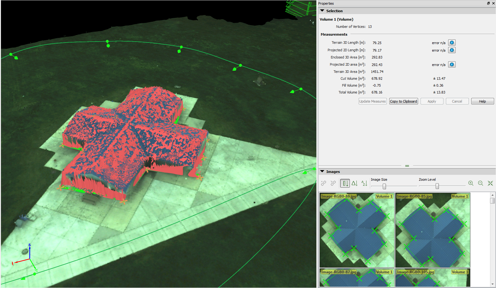
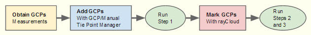
     Following the same basic sequence as the previous lab, images were loaded in to Pix4D. Although the images were geolocated we had GCP data and the coordinate system was known. Going off of that, Method 1 (Figure1) was used in order to add GCPs to the project. The program prompted a coordinate system to be selected and this is where NAD 1983 Zone 15 was chosen. The GCP/Manual Tie Point Manager (Figure 4) is a tool that shows the user the coordinates of each GCP and how many tie points have been manually adjusted. Once the GCPs are added run Step 1: Initial Processing, after that is a complete look at the Initial Processing Report and begin marking tie points. To tie points to the GCP a user has to go under rayCloud Editor and manually select tie points near the center of the GCP (Figure 5). Accuracy is based on the number of "ties" a GCP gets and for this lab at least 10 images were "tied".

Figure 4 - GCP/Manual Tie Point Manager showing how many tie points and location of each of our 6 GCPs

Figure 5 - Example of adding "ties" to images of GCP 5.

      Once the GCPs are tagged the image is prepped to be ran through steps 3 and 4. These steps can take anywhere from a couple of hours to a couple of days depending on how many images and GCPs the project has. It is crucial you make sure everything is set and ready to go before running the rest because you could potentially throwing out a lot of processing hours if do not select the right things. A good way to check your progress before running the last 2 steps is to examine the Initial Processing Report (Linked below). It addresses items such as quality check which essentially gives you an idea of how many images the project contains along with a some georeferencing and matching stats. There is also a preview included which is a glimpse of what is to come. If the preview is off, make sure you take care of what is missing before continuing. Also included are image position locations, GPS tie points, the amount of overlap and an overview of geolocation details which shows the level of error.

     For the sake of comparison the data was also processed without the addition of GCPs added. The results of the initial processing report for that can also be found linked below.

Initial Processing W/GCP
Initial Processing W/Out GCP

Results:
     Once the processing is complete you will be presented with a Final Report (Linked Below). This report expands upon the original Initial Report and updates needed values. As you can see the project containing GCPs has a much increased accuracy with drastically less amounts of error. The project with no GCPs has the same accuracy as the initial process states because the geolocation was not improved upon.

Final Report W/GCP
Final Report W/Out GCP

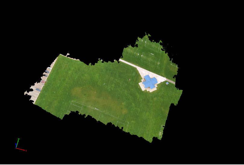
     Pix4D Also creates .tiff images that can be brought in to ArcMap. These can be placed over basemaps to give an updated image of your study area. This is where location accuracy is crucial. (Figure 6) shows the .tiff containing GCP data while (Figure 7) highlights what happens when your data integrity is not at it's fullest. As you can see in (Figure 7) the imagery tends to pull towards the Northeast, something adding GCPs corrected.

Figure 6 - Map with GCP data

Figure 7 - Map without GCP data

     A simple .gif image (Figure 8) comparing the two .tiff images is a decent indicator of the differences between the two. Although some may consider the differences minimal, when you are working with images that need to be geolocated correctly, a few meters is like night and day.

Similar to Pix4D in ArcScene, you can also "explore" the 3D model once adjusting the base heights for both the .tiff (Figure 9)  and .dsm. (Figure 10). These models give you an idea of the varying levels of elevation.

Figure 9 - .tiff with adjusted base heights in ArcScene 

Figure 10 - .dsm with adjusted bas heights in ArcScene

     Much like the last lab you can also "tour" your finished product. Below (Figure 11) is a tour highlighting each of the 6 GCP locations and also the study area as a whole.

Figure 11 - Video tour of 3D model created in Pix4D

While collecting data that day we also used a variety of other methods to see how accurate they were compared to the GCPs we laid out (Figure 12).

     There is truly so many ways the data can be manipulated and further processed but the above were a few key, basic items. All came from ArcMap, ArcScene, Pix4D.
Conclusion:


Again, Pix4D claims to be user friendly and the "help" guide proves itself time after time. If don't with time and care GCPs can be added in an efficient matter and can drastically improve the quality of your image. When adding "ties" the more you add the more "self aware" Pix4D gets and it begins adding ties for you. Alone, the SX260 does a decent job with geolocating but it is not at survey grade. This is why proper equipment and diligence is so important when working with precise imagery. This is still only scratching the surface of what Pix4D has to offer but going forward with the knowledge in regards to GCPs, our images will only improve with accuracy and the quality of the finished product will also improve.

Activity 7 - Pix4D

Overview:

     In past labs georeferenced mosaics have been mentioned but until now they have never been a true orthomosaic. Fortunately, Pix4D a UAS mapping software packages makes creating these extremely easy, and accurately. Although easy to navigate this software demands a lot of computer resources to process data quickly and has some guidelines such as in general your images should have 85% frontal overlap and at the very least 70% side overlap to be safe. Some terrains are more difficult than others such as snow and sand, to achieve the best results at least 85% frontal and 70% side overlap but also try and get adjust the exposure settings. With the right exposure you will be able to get the most contrast from each image.  Depending on the specs of your computer and how many images you are processing determines the time it will take to finish. Luckily, Pix4D includes a feature that allows you to view a preview, they refer to this feature as Rapid Check. This can save countless hours incase your data is not good and you wait for it to process sometimes for 12+ hours at a time. Rapid Check works by reducing the resolution of all your images to 1 mega pixel. This gives you not only a preview but gives you an idea of the quality level of your images. Whether or not the Rapid Check succeeds or fails is an indicator if you should move on with the project or collect data again achieving more overlap or a different method. Pix4D is also capable of handling multiple flights at a time. To do so the pilot has to make sure there is enough overlap and conditions remain as close as possible. For example, weather, sun direction, altitude, etc all need to be considered when handling multiple flights. While using Pix4D you are not just limited to using images shot in nadir, oblique images can also be used but there should be images taken from the ground as well and if you are capturing flat ground, nadir is recommended. Depending on your project you may want to use GCPs although these are generally optional. GCPs can be used to improve accuracy and is important to use if your sensor does not geolocate. During the various steps of processing a quality report is written. This gives the user an idea regarding the level of quality their project and if there are errors, what needs to be done in order to fix those errors.

Walkthrough:

     Although very user friendly Pix4D is a very powerful program with many uses. For this lab a very basic project was processed in order to introduce us to Pix4D and get us accustomed to the basic features. For this lab all of the images used were shot in nadir and it is important to note we did not use GCPs.

    When starting the program and a new project Pix4D prompts you to add images to begin processing. (Figure 1) Make sure to add all over your images in order to get a complete product.

Figure 1 - Adding Images to Pix4D

For this lab I processed two sets of images separately both featuring the Eau Claire Soccer Complex Pavilion shown in past labs.

     Once the images are added a screen will popup showing you the image properties. (Figure 2) Listed here are the coordinate system, if your images were geolocated or not and the camera/sensor used to take thos images. It is important to note, some sensors do not geolocate images and it is advised to supplement that through the use of GCPs or a georecording device that tracks points where images were taken.

Figure 2 - Image Properties Menu

     From there you are prompted with templates, this helps determine what direction you want to take the project. For this lab we went with the default 3D maps as you can see in (Figure 3)

Figure 3 - Project Template Selection

 

     Next, the processing begins, at this point its start and wait. Depending on the level of quality and number of images you have determines how long it will take for the entire process. The better of computer you have the less time it will take to process. Along the way, frequent process reports will pop up giving you quality updates and even previews of your final image/model.

     The quality report includes many useful things as mentioned earlier. One example is it shows you how many of your images were used in creating the finished product (Figure 4) and where your key areas of overlap were and were not. (Figure 5) In the case of the SX260 all of my images were used in creating the image.

Figure 4 - Beginning of Quality Report

Figure 5 - Overlap details

It makes sense my weakest areas of overlap were the outside fringes on the mission area. These areas were not the main focus of the mission therefor less images were meant to be taken.
     The first data I ran was from the Sony SX260, it was 32 images at 14 megapixels each. The SX260 geolocates images so I did not have to worry about that.  They were shot at 70m and in all it took around 30 minutes from start to finish to process. The other set of images I processed were taken by the GEMs sensor. There were 220 non-geolocated images so GPS data had to be added to maintain accuracy. Although there were many more images taken the GEMs only takes pictures at 1.3 mega pixels. This took slightly longer to process at around 40 minutes. The process for both the SX260 and the GEMs was nearly identical and consequently produced very similar results.

Post - Processed Data

     Once finished processing the data can be manipulated in a number of ways and almost "explored" much a like a virtual tour of the study area. A few of the basic features of Pix4D include, measuring features, find surface areas of objects and also some volumetrics. Because we are just getting introduced to Pix4D I used just those three tools. I measured the width of the sidewalk. (Figure 6), found the surface area of one of the soccer fields (Figure 7) and also the volume of the pavilion (Figure 8).

Figure 6 - Width of Sidewalk

Figure 7 - Surface Area of Soccer Field

Figure 8 - Volume of Pavilion

 You can also record an animation that "flys" you through the project. This is a relatively rough model given the fact we just used nadir images but gives a viewer a sense of the study area and can be made quickly. (Figure 9).

Figure 9 - Video Flyby Tour of GEMs 3D Model

With the processed data you are not restricted to just using the data in Pix4D. It can also be used and imported in to ArcMap. Here you can add metadata to your images, an important step in to ensuring data integrity. You can also create maps using the orthomosaic images  you created. (Figure 10, 11, 12)

Figure 10 - SX260 Orthomosaic made in ArcMap

Figure 11 - GEMs Orthomosaic made in ArcMap

Figure 12 - GEMs Orthomsaic with surface overlays from earlier calculations